Improve Sensitivity and Reproducibility using Pulsed Pressure Splitless GC Injection

In my previous blog, I discussed the possibility of backflash in Splitless GC Injection and its effect on quantitative reproducibility and carry-over.

Whilst much is written in the literature on optimisation of splitless injection conditions, little is available on the implementation and optimisation of increased head pressure (pressure pulsed) injection, so we will concentrate on this aspect of Injection Optimisation.

In most Split / Splitless GC injection systems there is a finite volume within the liner in which the gaseous sample needs to be maintained.  If the gaseous volume of the sample exceeds the liner volume, then backflash occurs and analyte may be deposited onto the non-heated surfaces within the septum purge, split and even carrier gas inlet lines leading into and out of the inlet.  Subsequent backflashed injections risk re-solubilising some of this deposited material and ‘pulling’ it back into the inlet and ultimately onto the column as the inlet empties under splitless conditions, thus contaminating the injected sample vapour.

The risk of ‘backflash’ can be assessed using simple calculators into which the GC inlet operating parameters are entered along with some information on sample solvent and injection volume and an assessment is made of the vapour volume created on injection against the available internal volume of the inlet liner used.

Analysis conditions and backflash assessment for injection of a predominantly aqueous sample is shown in Figure 1.

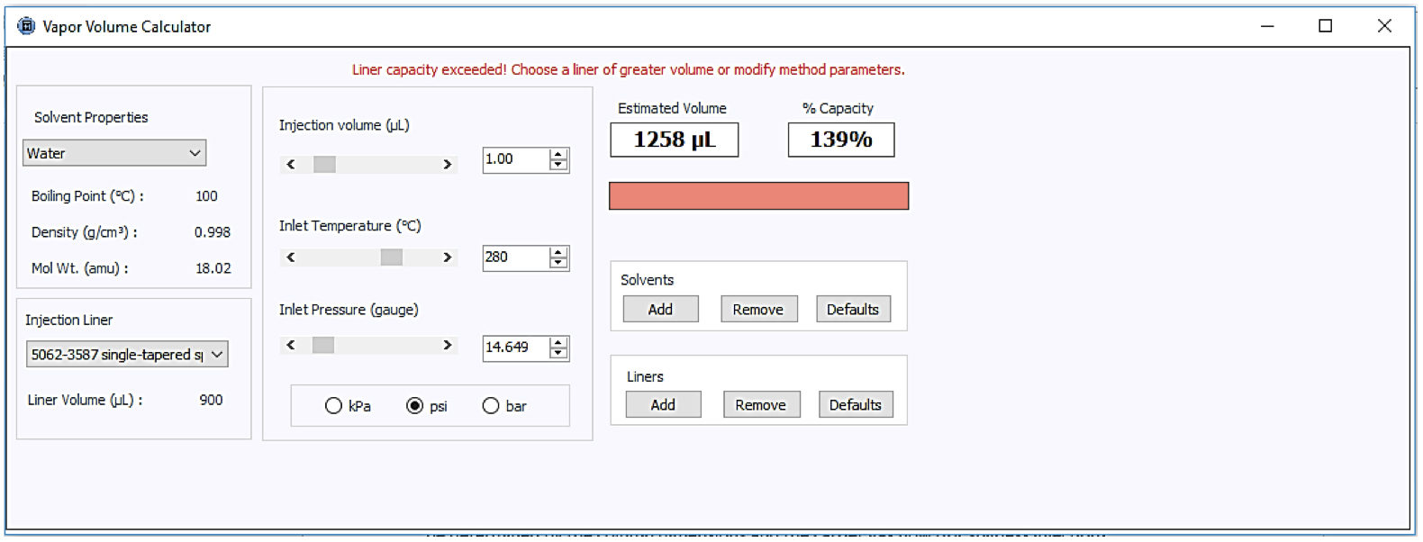
Figure 1: Vapour volume calculation for a 1mL splitless injection of an aqueous sample.
(Courtesy of Agilent Technologies, Santa Clara, USA) https://www.agilent.com/en/support/gas-chromatography/gccalculators)

Note: inlet pressure can be found from the instrument software or instrument front panel and will be determined by the column dimensions and the carrier gas flow (for splitless injection).  Alternatively this pressure may be calculated using an offline calculator, again based upon the required column flow and column dimesions.
(See here for a pressure / flow calculator  https://www.agilent.com/en/support/gas-chromatography/gccalculators)

In the above example, the liner volume is exceeded by the volume of sample vapour created and therefore there is risk of backflash and carry-over, leading to potential contamination and quantitation issues. Sample solvents with high expansion coefficients, such as water, are particularly problematic as small injection volumes lead to large vapour volumes.

Obviously one way to overcome these issues is to inject a lower sample volume, however in splitless injection, which is typically used for the analysis of trace analytes, this may lead to an issue with the detectability of analytes and sensitivity of the method.  An alternative way to overcome backflash is to reduce the volume of sample vapour which is created during the injection by increasing the pressure within the inlet which constrains the expansion of the sample.  This is known as ‘pressure pulsed’ injection and the incre0ased pressure applied within the inlet is typically reduced prior to the end of the splitless period to re-establish the required pressure / flow through the column for the analysis.

With this approach in mind, a further assessment may be made to identify the inlet pressure required to constrain the vapour volume created with our 1mL aqueous sample injection to within the available volume of the inlet liner – as shown in Figure 2.

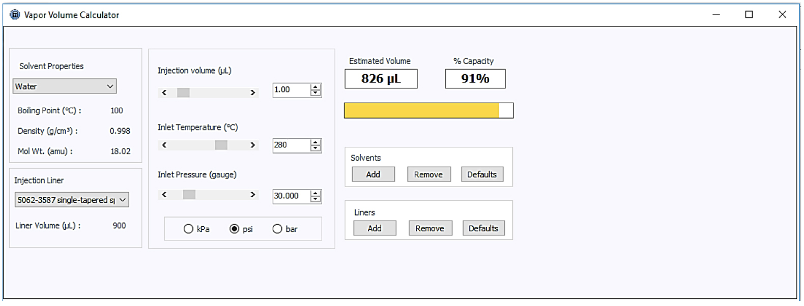
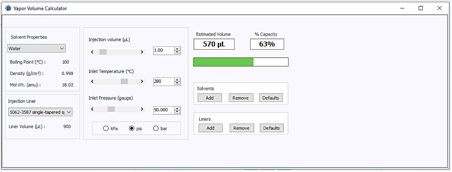
Figure 2:  Vapour volume calculator used to assess the inlet pressure required to contain the vapour created from a 1mL injection of an aqueous sample under the conditions outlined in Figure 1.

Figure 2 indicates that an increased head pressure of between 30psi and 50 psi (typically the upper limit of the pulse pressure available in most systems) would lead to the solvent vapour volume being constrained within the liner and therefore a reduced possibility of backflash and carryover.

The implementation of pressure pulsed injection requires the addition of two further variables (1 and 2 below) to the splitless injection method which now typically must define;

1. Pressure during the injection phase (pulse pressure)
2. Time of the Pressure Pulse
3. Splitless Time / Purge Time (time at the which inlet is switched from splitless to split mode in order to empty the inlet of excess residual solvent vapours)
4. Inlet Pressure (post pressure pulse) required for sample analysis

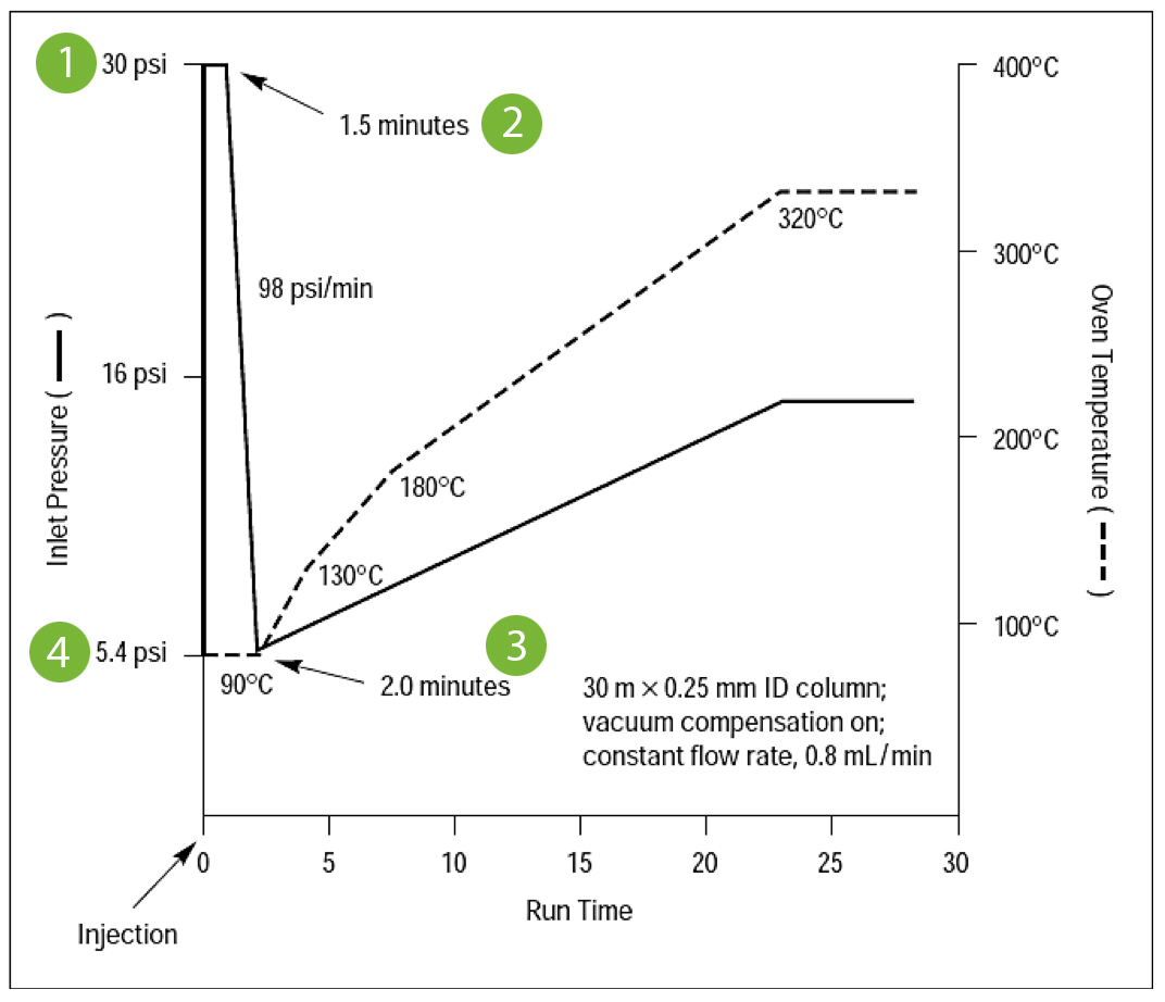
Figure 3: Pressure / Temperature timeline for a typical pulsed pressure splitless injection (Courtesy of Agilent Technologies, Santa Clara, USA)

It is important to note from Figure 3 that there is a finite time required to move from the higher pulse pressure to the pressure required for the analytical separation and even though the rate of pressure reduction is high (98psi/min.) this will still take 15 seconds to recover from a 30psi pulse to the 5.4psi required for the analysis.  Careful consideration is required in setting the pressure pulse time in relation to the splitless time (time at which the split vent is opened) as, in our experience, the relationship between the pressure pulse end time and the splitless time can be critical in determining the reproducibility of the injection.  In some cases it is more favourable for the split to be opened whilst the pressure is high, and the pulse time relative to the splitless time often requires some empirical optimisation.

Figure 4 shows chromatograms resulting from splitless and pulsed splitless injections of an aqueous sample containing 5% Dimethylformamide (aq) followed by a water ‘wash’ injection and a subsequent ‘standard’ injection containing ethyl hexanol (5.55mins.) and benzaldehyde (6.15mins).

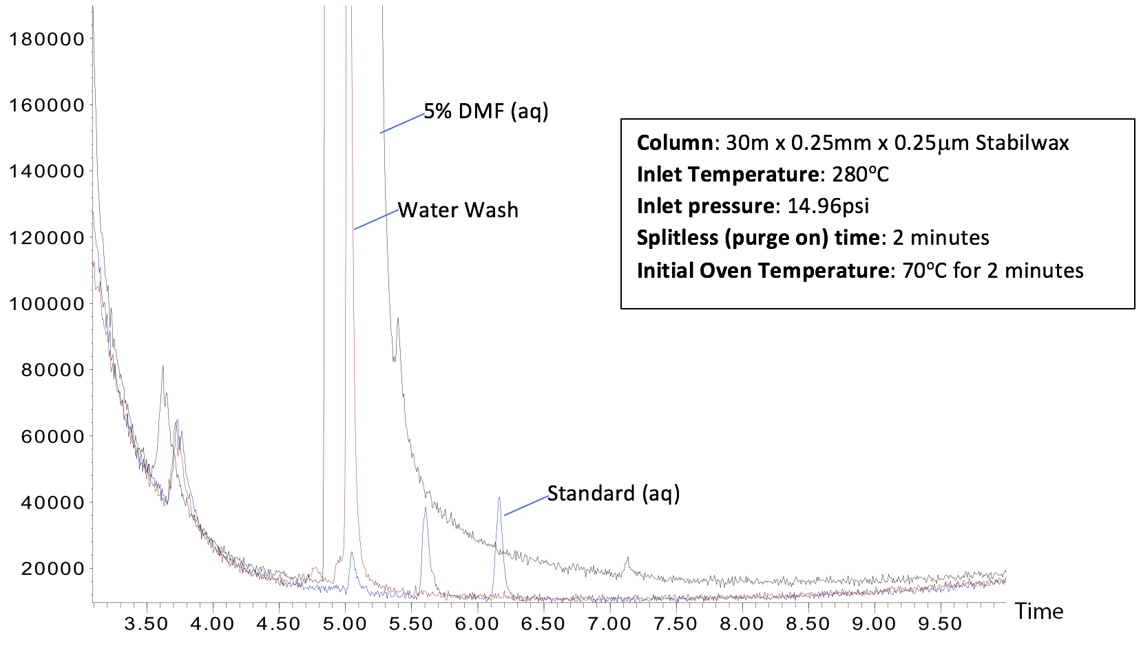
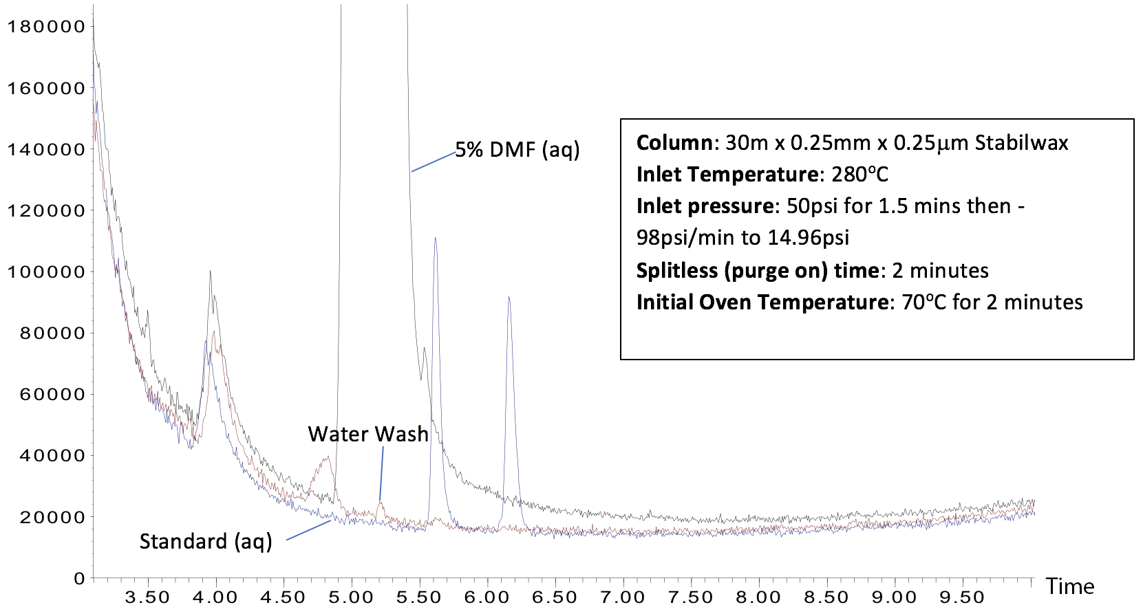
Figure 4: Splitless Injection (Top) and Pressure Pulsed Splitless Injection (Bottom) of a 1mL injection of an aqueous sample containing DMF followed by water wash and standard injections.  Bottom injection has a 50psi pressure pulse from 0 to 1.5 minutes with a 2.0 minute splitless time.

The top chromatogram of Figure 4, generated using standard splitless conditions, shows a large amount of carryover of the dimethylformamide (retention time 5.05 mins.) in both the subsequent water wash and the ‘standard’ chromatograms.  In the bottom chromatogram, a pressure pulsed injection of 50psi for 1.5 minutes with a 2 minute splitless time is used to reduce carryover.  Whilst there is a very small amount of DMF carryover into the Water Wash injection, this is an extremely challenging application example and the amount of carryover is drastically reduced in comparison to the standard splitless experiment.  The subsequent ‘standard’ injection shows no trace of DMF.

It is very important to note that when using pressure pulsed injection, the usual rules of splitless injection apply and it is important that the initial oven temperature is at least 10^oC below the boiling point of the injection solvent to allow for good peak focussing,  Further, the initial hold time for the oven temperature may require some empirical optimisation in order to derive the best peak shape/ efficiency, however the hold time should not be any less than the splitless time.

Under some circumstances, peak slitting may be observed when undertaking pulsed pressure injection which can be attributed to the rapid change in pressure at the end of the pressure pulse.  If this occurs, first extend the time between the end of the pressure pulse and the splitless (purge-on) time and if unsuccessful, alter the ramp rate of pressure reduction at the end of the pressure pulse from 98psi per minute to 20 psi per minute and lengthen the splitless time commensurately.    The use of a retention gap (1-3m) of fused silica prior to the analytical column may also help to reduce the effects of peak splitting.

It is also recommended that the inlet septum is changed regularly in order to avoid analyte losses during sample addition into the inlet under the increased pressure conditions.  Whenever pressure pulsed splitless injection is implemented, one needs to not only assess the reduction in carry-over, an assessment of the precision of analytes of interest should also be made to ensure appropriate conditions have been selected.  Figure 5 (top) shows the assessment of repeatability using the pressure pulsed injection conditions of Figure 4, clearly highlighting variability of peak area of the ethyl hexanol and benzaldehyde peaks.  By shortening both the pressure pulse and splitless times (liner clearance time can be calculated at 0.18 mins), this variability is eliminated to within the required reproducibility requirements.

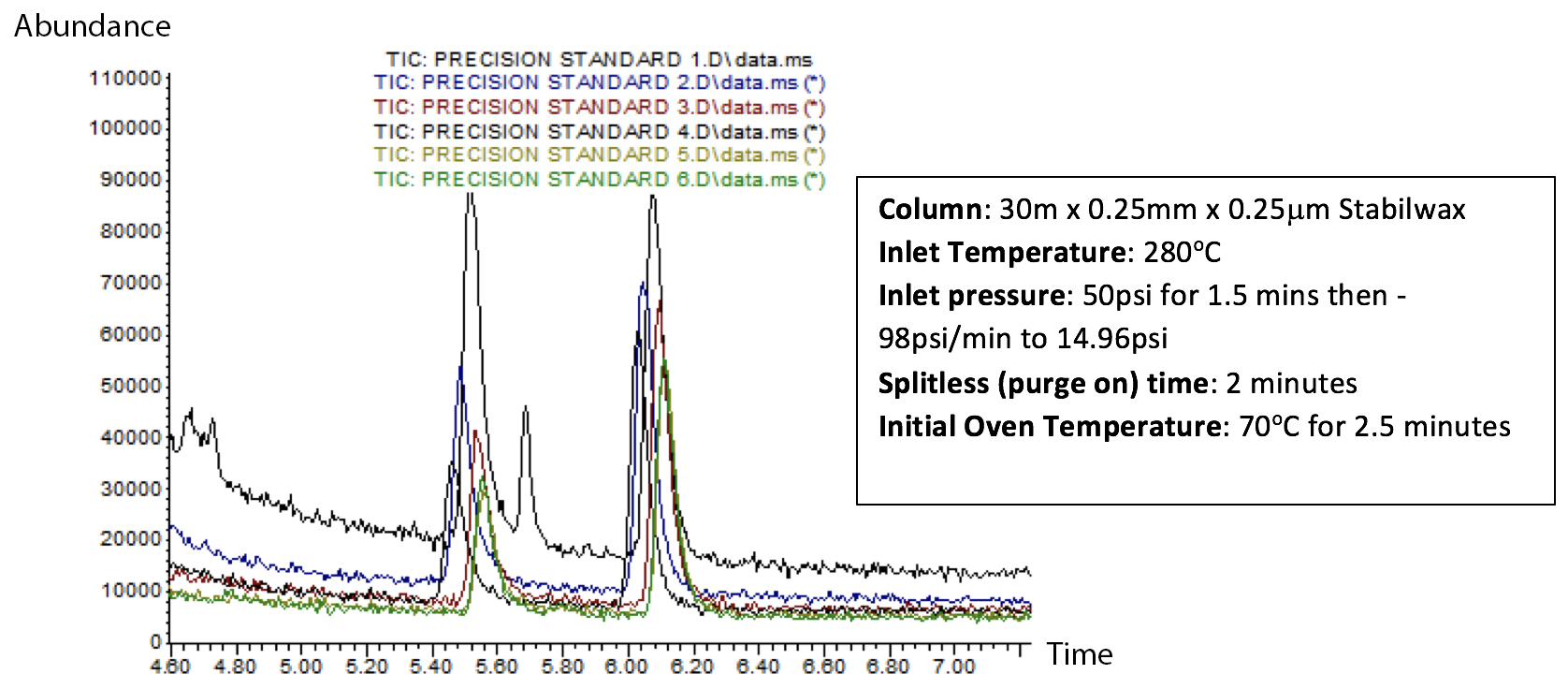
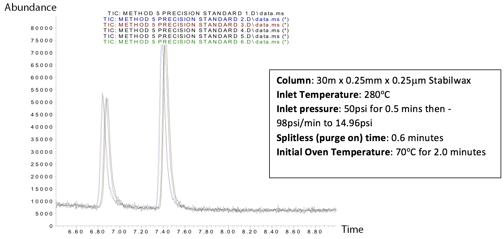
Figure 5: Improvement in reproducibility through empirical optimisation of pressure pulse time and splitless time.